AIRCRAFT SCATTER (ACS)
Introduction
Aircraft scatter is the process of scatter radio waves of the body of a traveling aircraft in order to enhance the distance possible to bridge on VHF, UHF and microwaves. We will call aircraft scatter "ACS" in this context.
ACS will give you the possibility to work VHF-UHF DX independent of weather conditions.
If you are a VHF - UHF ham operator, you have probably experienced ACS already. Even if you do not have worked a QSO via ACS you may have heard that DX station (<800 km distant) for just a fraction of a minute and then disappearing. Another effect is that if you are listening to a signal in the 200 to 400 km range that suddenly starts to fade violently with a fair amount of signal strength enhancement. After less then a minute the signal is back to the low troposcatter signal level again. Both of these situations are with good chance effects of ACS. If you understand the nature of ACS, it can of cause be used to make QSO's with distant stations.
Although known for many years, ACS has not been exploited to its full potential in an efficient way until recent years. See ref. [1] and [2].
On this web page I will try to explain some of the mechanisms behind ACS. My intent is to increase the interest and usage of ACS. I also provide some help to calculate the main parameters for an ACS communication link.
The ACS path
Aircrafts are traveling up to an altitude of 10 000 meters or more. The altitude of the aircraft determines the maximum distance possible to span. They travel at a speed up to 1000 km/h. This gives a maximum possible Doppler shift on the scatter signal.
In the RADAR literature you can find the expressions mono-static and bi-static RADAR. Mono-static means that the Tx and Rx are at the same site (location). Bi-static means that the Tx and Rx are NOT at the same site. ACS is a case of the bi-static situation. Also when discussing RADAR you use the expression Radar Cross Section (RCS), in the meaning of the apparent size of a target in square meters for radio waves. The RCS varies with the wavelength of the radio wave. The RCS is not the same as the physical size of the target (aircraft) but the size it appears to be when reflecting radio waves. The RCS is of cause dependant of the physical size of the target, but also of the way the target looks. One example is the stealth aircrafts that has a small ACS compared to its physical size, at least in some directions and aspect angles. The RCS can differ largely with aspect angle, i.e. how the radio wave hits the aircraft (rear, front, side etc.) The RADAR literature states that the bi-static RCS in general is much larger than the mono-static. This is in favor for HAM ACS.
The most common path for HAM ACS QSO's is probably when the aircraft is at or very close to the great circle path between the two stations involved. From station A to the aircraft you have a path loss. At the scattering from the aircraft you can have a loss or a gain, depending on how the radio wave spreads or forms a beam. In some direction the radiation will be enhanced by the form of the scattering body of the aircraft. The last part is the path loss from the aircraft to station B. The total path loss is the sum of these three terms. In order to get a useable signal from station A to station B via ACS, the total station performance (transmitter power, antenna gain and receiver noise figure) must be greater than the total path loss.
The actual Doppler shift is in most cases much lower than the calculated maximum possible Doppler shift. This is due to the fact that both stations does not experience the maximum aircraft speed in the same direction (ascending vs. descending) simultaneously unless they are at or very close to the same site i.e. beaming in the same direction to hit the aircraft. If the aircraft crosses the great circle path between station A and station B at an right angle, the Doppler shift will be close to zero as the aircraft does not have any radial speed when the crossing is made. This is clearly visible in Fig. 3 and Fig. 5 where the ACS trace crosses the tropo trace of SK7MHH and OZ7UHF respectively. If the aircraft is traveling along the great circle path between station A and station B the signal will have a negative Doppler shift chasing the aircraft from behind and a positive Doppler shift leaving the aircraft in the other direction. The positive and negative Doppler shifts will cancel each other to a large extent and the remaining Doppler shift will be low. As seen in Fig. 3 and Fig. 5, the real world ACS Doppler shift on 70 cm is a few hundred Hz. The experienced Doppler shift at higher bands will be scaled with frequency i.e. three times larger on 23 cm, five to six times larger on 13 cm and so on. On lower bands the Doppler shift will be scaled down with frequency in the same way.
Equipment requirement
Here is a simple, Excel based, path loss calculator to use for calculating your stations capability (beta version). It assumes line of sight, free space path loss conditions. The models that the calculations are based upon are not accurate to the single dB, but will give you a good understanding of what equipment that is needed for ACS communication on the VHF, UHF and microwave bands. It also calculates the maximum possible Doppler shift to expect for a specific operating frequency and aircraft speed. The models seem to give accurate results on the UHF bands (70, 23 and 13 cm) and somewhat pessimistic results on the microwave bands (6 and 3 cm).
The calculator estimates:
- The Free Space Path loss between isotropic antennas for the distance given.
- The total Path loss the two stations described can bridge with 0 dB S/N ratio.
- Signal level in dBm at the receiving end for Free Space Path loss.
- Signal to noise ratio at the receiving end for the ACS scenario.
- Maximum Doppler shift for the frequency and aircraft speed used.
- Approximate Beam Width (degrees) for the antenna gain given.
- Approximate Beam Width (in kilometers) at the aircraft position.
- Minimum time for the aircraft in the beam for the aircraft speed used.
- Approximate azimuth and elevation Beam Width of the optimum scatter beam from the aircraft.
- The maximum distance for line of sight (LOS) to an aircraft as function of the cruising altitude of the aircraft. Two times this distance is the maximum distance from station A to station B for LOS to the aircraft. The effect of local obstacles is not taken into account.
- Approximate aircraft elevation angle seen from both ends of the path.
The calculations are made using the following assumptions:
- There is line of sight (LOS) from each station to the aircraft.
- The signal level calculated assumes the maximum realistic that can be obtained. There is a certain statistical process involved, that actually all factors coincide and gives this scatter gain.
- The aircraft is assumed to act as a radiator of its physical size with certain efficiency (50%).
- The scattering properties of the aircraft are identical for both the A to B and B to A paths.
- The antennas have equal beam width in azimuth and elevation. This means that e.g. vertical stacks will not be represented in a correct way.
A few conclusions can be drawn by using the calculator:
- It is favorable for the path loss that the aircraft is close to one end of the path.
- On 70 cm (432 MHz) you can get satisfying results with 100 W and a single yagi, up to at least 500 km.
- You need one of the big aircrafts like 737, 747 etc. to get good signals. Small 4 seats, one propeller aircrafts just won't do it.
- The resulting beam from the aircraft is very narrow and will together with the movement of the aircraft determine the timeframe that is available for the QSO.
- The same antenna size, e.g. a 1.6 m dish, will give better gain on a higher band (e.g. 13 cm vs. 23 cm) and compensate for the higher path loss on the higher frequency band (with all other radio parameters, Tx power, Rx sensitivity, Rx band width etc. remain the same). In addition the "gain" from the aircraft will increase with frequency and produce better signals but the "beam width" of the aircraft decreases with frequency and the time available for a QSO will decrease on a higher frequency band.
- As always, the better the take-off of the QTH is, the better the results will be.
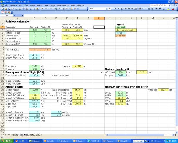
Figure 1. Screen dump of the Excel calculation sheet.
Operating techniques
The time available when an aircraft is in the right position, gives propagation for usually less then one minute. This calls for a working QSO procedure. Use a calling sequence of 15 seconds for each station. Exchange only the most vital information for the QSO. Do not repeat every piece of information several times.
Using the time tables available from the different air carriers and airports, can be of great help in planning the skeds and operating times. Especially if you live in the neighborhood of an airport, using the time tables can be very efficient. When working in the direction of the airport landing and take off can be useful for ACS, even if the height of the aircraft is not that great. One such source of information for
My experience from the airport of Landvetter, about 40 km distant in 35 degrees azimuth, is that I can work stations from 30 to 60 deg in azimuth 5 to 15 minutes before scheduled arrival and 5 to 15 minutes after scheduled departure seams to work with rather good rate of success. In spite of the lower altitude of the aircrafts ascending to and descending from the airport, it works fine up to distances over 500 km on 23 cm.
Results
The first time I used ACS intentionally was in 1993 when working SM5BEI (JP81) on 23 cm over a path length of 521 km and SM5CTV (JO88) in 1994, also 23 cm over a path length of 283 km (very bad horizon at SM5CTV). In 1996 SM6CEN/4M in JP71 was worked on 70 cm over a path length of 452 km. The equipment for these QSO's was not extremely sophisticated at neither end.
ACS was regularly used by SK6YH in the 23 cm Scandinavian microwave activity contests in 1995 to work SM5BEI at 521 km and a group of SM5/SM0 stations at 400+ km.
Today ACS is used on an regularly basis from 23 cm to 3 cm to work at least 500 km in the monthly Scandinavian microwave activity contests by several stations.
From my winter QTH in JO67AQ (with quite bad horizon in most directions), I can at a daily basis use ACS to hear both SK1UHF and OZ7IGY on 70 cm. I use very modest equipment: IC-706MkIIG with no external pre-amp, 6 element yagi in fixed direction (abt 135 deg az) only 4 m above ground. On top of that I have a neighbor (< 30 m away in 90 deg az) with four 434 MHz controlled light switches that produces a white noise of at least 10 dB above the normal noise level in my receiver with my antenna in 90 deg az. The antenna direction of 135 degrees is right at the southern approach / descend path for the aircrafts entering or leaving the
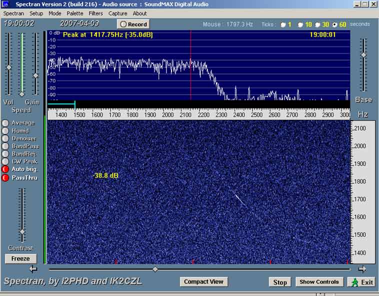
Figure 2. ACS trace from SK1UHF (432.404 MHz).
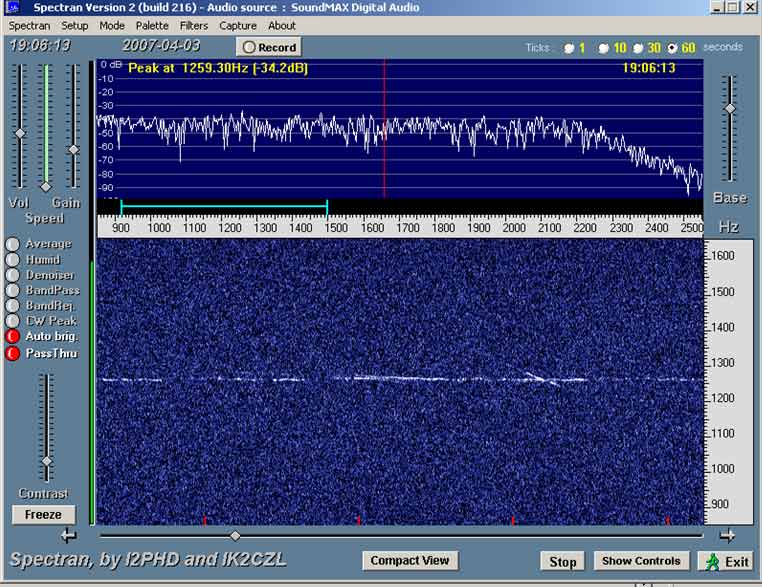
Figure 3. Tropo and ACS trace from SK7MHH (432.439 MHz)
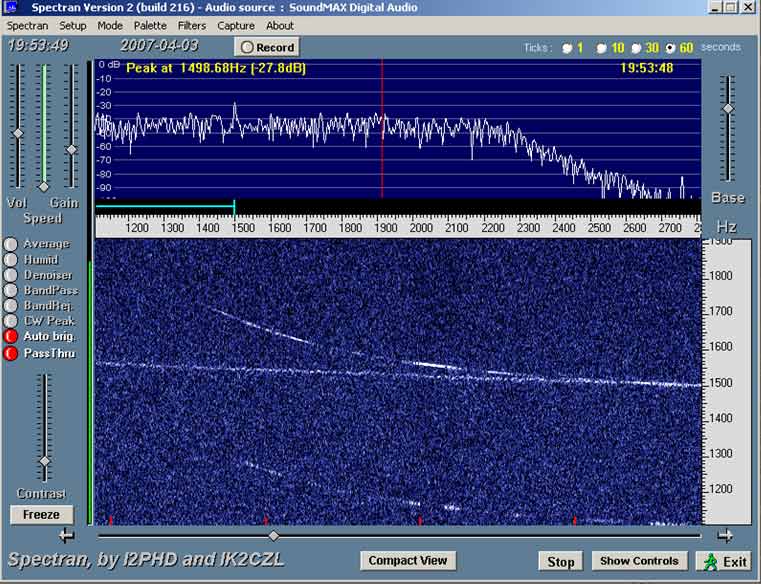
Figure 4. ACS trace from OZ7IGY (432.471 MHz). You can clearly see the beacons FSK of 400 Hz (space 400 Hz below mark). The straight trace is a artifact from my electronic neighborhood.
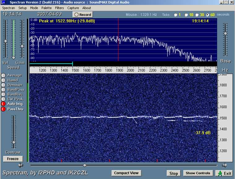
Figure 5. Tropo and ACS trace from OZ1UHF (432.447 MHz)
ACS is not limited to the UHF and microwave bands. It works fine on 50, 70 and 144 MHz as well.
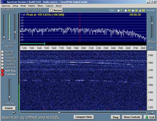
Figure 6. ACS trace from OZ7IGY on 50.021 MHz. You can clearly see the FSK space 300 Hz below the mark. The antenna used for this recording was a 5/8 lambda vertical (omnidirectional!!) antenna.
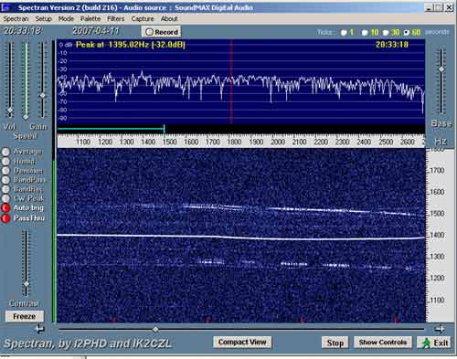
Figure 7. ACS trace from OZ7IGY on 70.021 MHz. You can clearly see the FSK space 250 Hz below the mark. The antenna used for this recording was a 1/4 lambda vertical (omnidirectional!!) antenna. The strong trace in the center is a artifact from my electronic neighborhood.
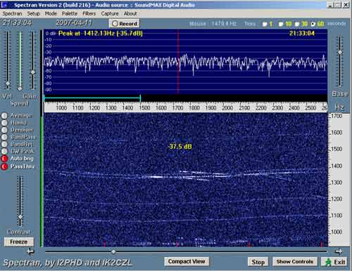
Figure 7. ACS trace from OZ7IGY on 144.471 MHz. You can clearly see the FSK space 400 Hz below the mark. The antenna used for this recording was a 1/2 lambda vertical (omnidirectional!!) antenna. Some of the weak traces are artifacts from my electronic neighborhood. You can also see that there are more the one reflecting aircraft with different doppler shift, actually three in parallel in the middle of the picture.
Above images were caught with Spectran while monitoring each beacons frequency. The receiver was set to USB and the displayed frequency was set to get the received signal at about 1500 Hz. The bandwidth of Spectran was set to 2.7 Hz. Each time tick (red) on the screen is one minute.
G3JKV has an article in RadCom March 2006 with an analysis of ACS.
G3XDY writes in RadCom April 2006 that he has worked stations up to 850 km away on 1.3 GHz ACS.
Links
Regrettably, there is not much to be found about ACS on the web. I hope the situation will change and more web sites dealing with ACS will pop up! These are the one I have found. Please give me info if you know any other.
[1] The following link will give more info about ACS experience in
[2] G3JKV writes about ACS on 144 MHz in http://www.lsear.freeserve.co.uk/aircraft%20scatter.html
[3] SM0DFP, Per, describes how to use flight data available on the air for improved ACS and the results from his work: http://sk0ct.se/propagation/flygscatter1.htm
[4] Aircraft transponder data from “Pilotmagazinet” http://www.pilotmagazinet.se/radar.asp
References
[1] QST July 1984, VHF/UHF world by W1JR Joe Reisert. The VHF/UHF primer: an introduction to propagation.
[2] ARRL UHF-Microwave handbook.
@ This page is under development and the links may not work as expected. The content of the text will also be updated. Check again soon and they can be updated!
![]()
Updated April 5, 2008. http://www.2ingandlin.se/SM6FHZ.htm